In this work, we seek to quantify the “common” or “typical” movements involved in oral sex performed on males. To do so, we analyze a dataset containing over 108 hours of pornographic video, annotated at each frame with the position of the lips along the shaft of the penis. We use quantization techniques to discover sixteen distinct motions, and using these motions we design and evaluate a system that procedurally generates realistic movement sequences using deep learning. We quantitatively show that this system is superior to simple Markov Chain techniques.
To our knowledge, this kind of analysis of pornographic content has never been done before. Results from this analysis lay the ground for future research.
This study was commissioned by Very Intelligent Ecommerce Inc. as part of the design of the Autoblow AI. The authors of this paper have chosen to remain anonymous.
Machine learning and big data analysis are becoming increasingly important in the digital world. The sex industry is no exception. For example: the exact same techniques used to filter out porn can easily be adapted to classify and tag it. Streaming sites also use Netflix-like recommender systems to recommend videos. These are only some of the practical applications of AI.
To our knowledge, though, there is a dearth of in-depth analysis of the content itself. In this work, we begin an investigation into this unexplored space, focusing specifically on oral sex performed on a male (“blowjob”). We investigate a dataset containing approximately 108 hours of pornographic video depicting blowjobs, annotated with the position of the lips along the shaft of the penis.
First, we quantify the most “common” or “typical” motions present in a blowjob, in order to improve the realism of the patterns used by the Autoblow AI. We use quantization techniques to identify sixteen “typical” or “common” movements, which are used as building blocks to build more complex movements.
Second, we use the results from the previous to investigate procedural generation of movement sequences, as an additional improvement available to future versions of the Autoblow AI. We design a system, based on deep learning, for generating unique but realistic sequences from random noise. We compare this system quantitatively against a simple Markov chain model to justify the design.
Finally, we discuss future research that is possible with the same dataset, in the context of continuing to improve the Autoblow AI and sex toys in general.
1145 pornographic videos depicting blowjobs were acquired and cut to contain only the sections depicting the blowjob itself. These clips were then manually annotated by reviewers, using a custom UI to record the position of the mouth along the penile shaft. The position was recorded as an integer, where 1000 represents the tip of the shaft, and 0 the base of the penis.
For analysis, the video and annotations were normalized to 16 frames per second using linear interpolation. The final dataset contained 6270467 normalized frames split into 1060 clips, totalling almost 109 hours of video.
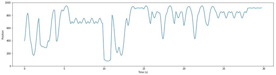
To follow this analysis, it helps to have a basic understanding of how the Autoblow AI is programmed, which heavily informs our approach and terminology. The Autoblow AI has tenmodes, each of which represent a sequence of movements. Amovement is simply a series of up/down motions at varying speeds, which are translated into motor movements. Two or more movements are concatenated to create a mode. Three example movements, and a mode based on them, are illustrated below:
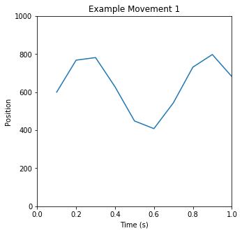
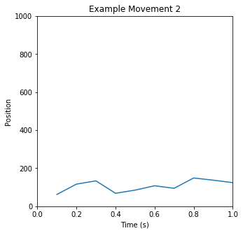
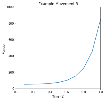
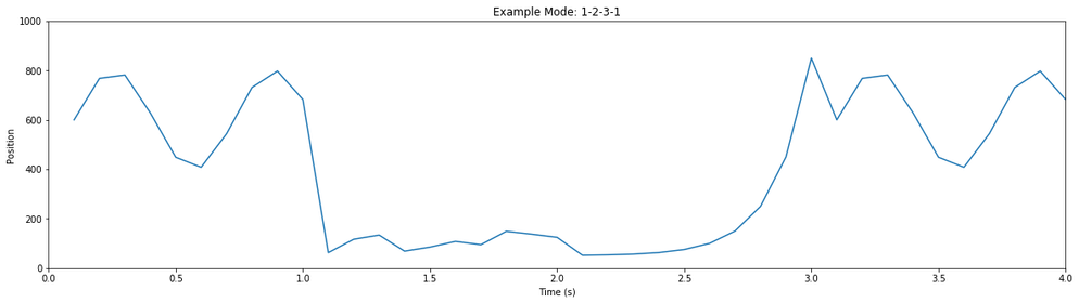
You can clearly see periodic motions happening; you can also see changes over time in the activity, as well as pauses and breaks. Based on manual evaluation of a thousand such snippets, our intuition was that we could identify “common” or “typical” movements in the data - building blocks from which we could construct the many modes of the Autoblow AI. The next step, then, was to validate and quantify that intuition.
We began our investigation with the venerable K-Means algorithm, also known as Lloyd’s algorithm. This algorithm has quite a few drawbacks; but it’s quick to set up and quick to run, and therefore a good “first shot” that informs later analysis. 1
We split each video into one-second windows; taking the sequence of positions for each window gives a set of 16-dimensional vectors. We then applied K-Means to find 16 clusters. The resulting means, and 100 samples for each cluster, are shown below:
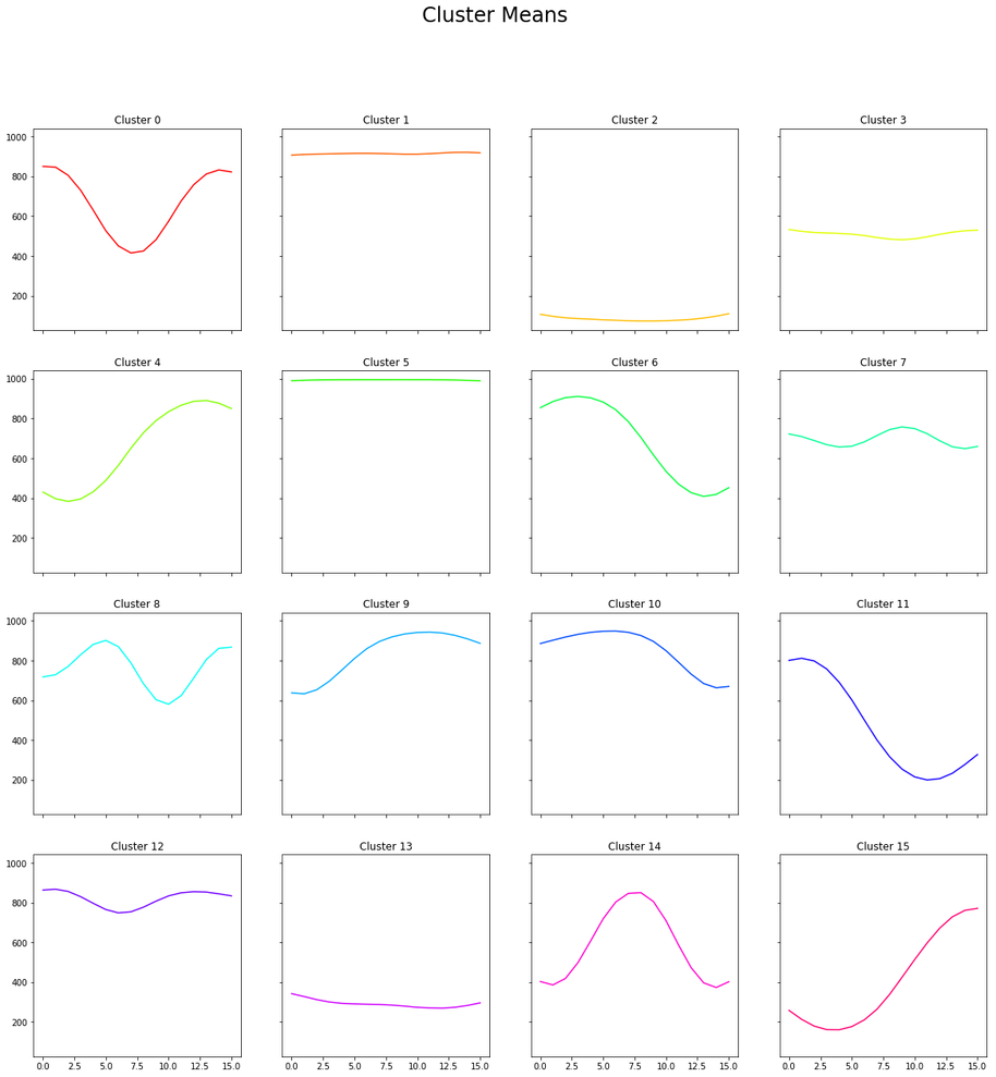
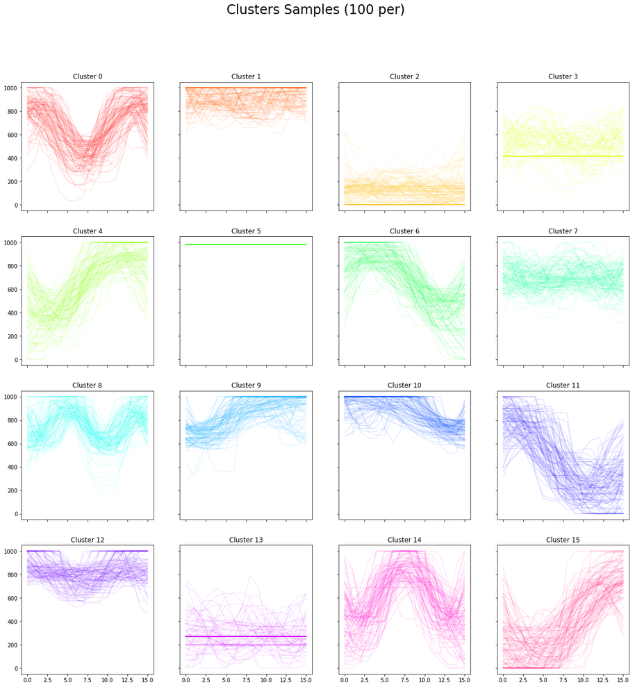
The results were better than we hoped. We managed to pick out little-to-no activity (associated with pre- and post-blowjob segments, pauses, edging); shallow activity near the top (tip play); concentrated activity near the base (deepthroating); transitions from top to base or base to top; and various variations on constant activity at various levels, and various frequencies.
To further validate our assumptions, we used a recently-developed dimensionality reduction technique known as UMAP to reduce the clusters to visualize the data in 2 and 3 dimensions.
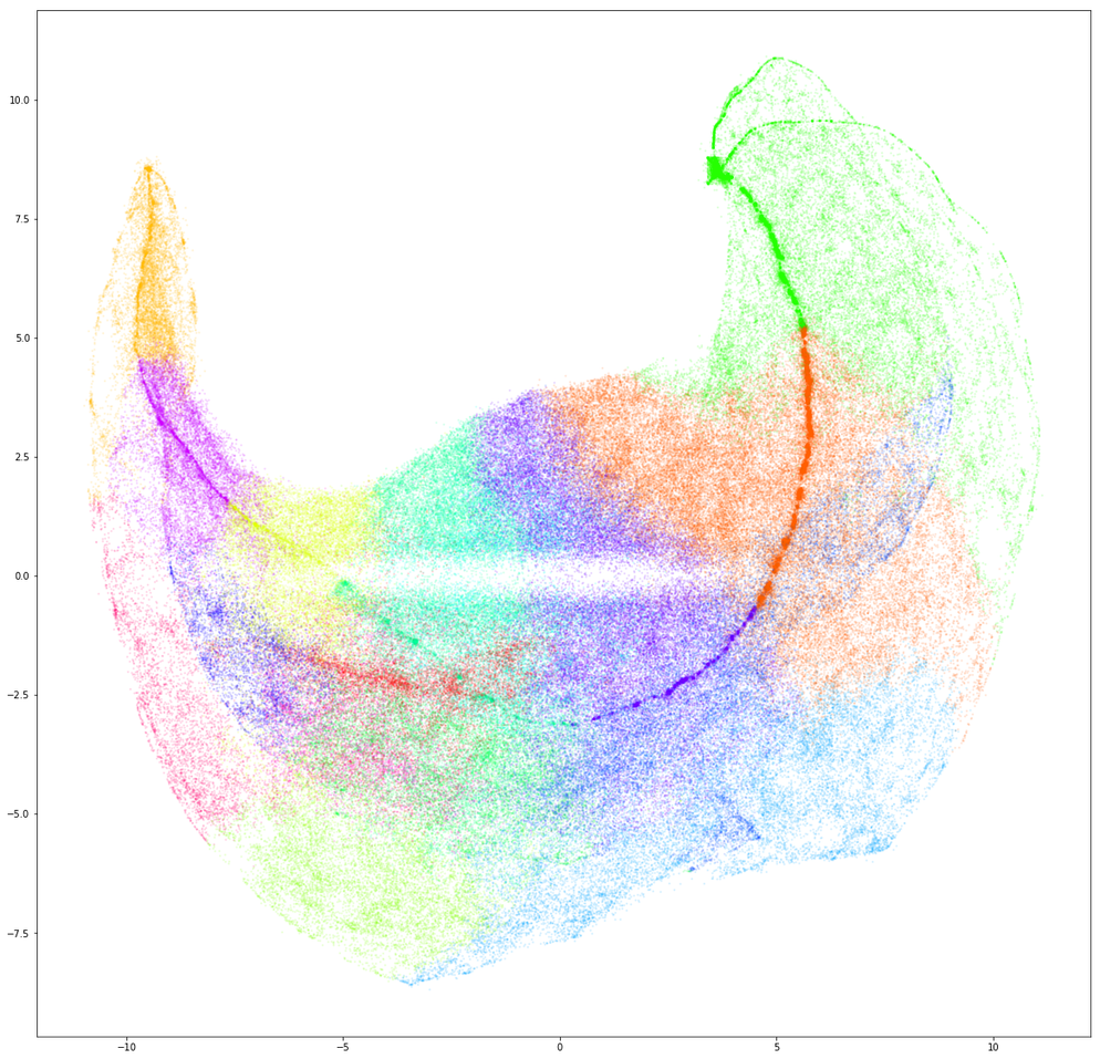
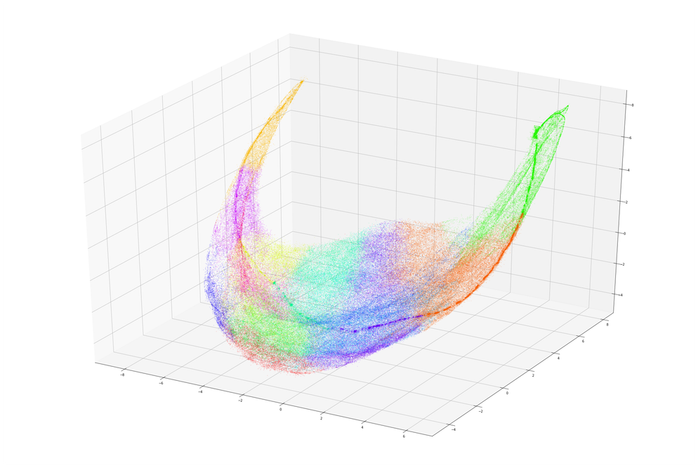
What we see actually has a lot of fascinating structure. Notice how data from clusters 5 and 2 - which represent little activity near the top and bottom, respectively - are located at opposite “points”. Notice too that clusters 1 and 5, which both represent light activity near the top, are next to each other. There’s also the dense line that runs between the “points” at each end, which generally seems to run through all of the clusters that represent low-magnitude activity (5, 1, 12, 7, 3, 13, 2), from highest to lowest center of activity.
We could spend a lot of time analyzing this graph, but for now this is enough to give us confidence that our “building blocks” are representative of strong trends in the data. We can now confidently use these to building up more complex sequences, or modes.
A full mode, as described above, is created from a series of movements. In the previous section, we identified common movements that occur in one-second intervals. A full mode, as described above, is created from a series of movements. Thus, the next step is to find common sequences of movements.
This problem bears a lot of similarity to natural language problems - particularly “guess-the-next-word”. The problem is best illustrated bythe following XKCD comic:
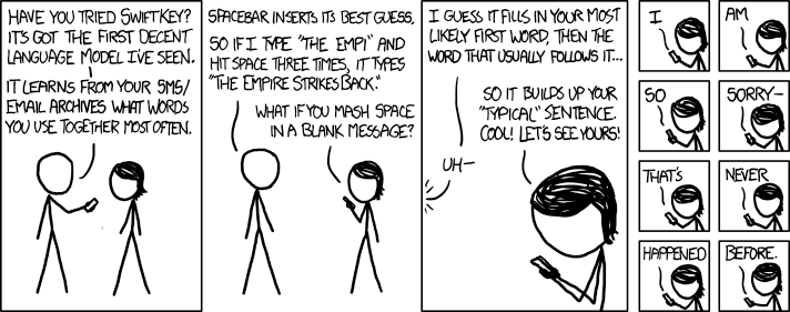
The problem here is very similar - we wish to build up a “typical” blowjob from the building blocks we established in the previous section. Thus, we can use similar techniques. We begin by creating a simple model based onMarkov chainsas a baseline. We then design a deep-learning model as an alternative, and compare the two quantitatively.
The idea behind a Markov chain is simple: we assume that where we go next only depends on where we are, not where we’ve been. For example, suppose we just did movement 1; and based on that, we know there’s a 50% chance that we’ll do movement 1 again, a 30% chance we’ll do movement 2 next, a 15% chance we’ll do movement 3, and so on and so forth. Then, we can generate a “unique” sequence based on this knowledge by randomly selecting the next movement at each time step, based on the probabilities.
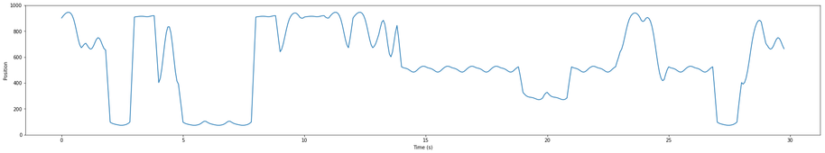
So, we counted the frequency with which each mode was proceeded by each other mode, and verified that the probabilities we saw matched our intuition. We then used these probabilities to generate unique sequences, and smoothed them out using a simple moving average. The results are shown below:
There’s just one problem with the Markov model; and it’s precisely the assumption that makes it easy to implement and effective in practice. The assumption beneath the Markov model is that the next-state probabilities are only dependent on the current state. In truth, they might be dependent on any number of previous states.
For example: suppose we start with the “no activity” state. Most of the actual data in the video starts in this state and stays there for some time. Under the simple Markov model, the probability of staying in this state is very high, and therefore it can “stick” there for almost arbitrary lengths of time; when in reality, we probably want to increase the probability of transitioning into a different state the longer we stay there.
In theory, this can be overcome by redefining the “current state” to be a concatenation of the (n) previous states. The problem is that the number of possible state combinations quickly gets out of
hand. For a length-1 state, we have 16 possible current states, and 16 possible next-states, for
(16 ∗ 16 = 256) possible combinations. For a length-2 state, we have
(16 ∗ 16 = 256) possible current states, and 16 possible next states, for
(16 3 = 4096)
possible combinations. In general, for a length- (n)
current-state, we have
(16n + 1)
possible combinations of current and next state. The dataset needs to be large enough that our samples can adequately
represent all of those possibilities; this may require an impossibly large dataset.2
This also has another problem: it requires us to know the “optimal” number of previous states to perform the prediction. In practice, this might vary; if the last 3 states were A, B and C, maybe it doesn’t really matter what happened before that; but maybe if they were X, Y and Z, it does. This is only implicitly captured by the Markov model. There may also be very complex correlations in play that aren’t obvious to humans.
Whenever the phrase “complex and non-obvious correlations” comes into play, that’s a good sign that we want to start looking at deep learning.
In this section we design a dense neural network (DNN) architecture that predicts the next state based on the previous states.3
We use a simple two-layer architecture, whose input is the last 16 states, and whose output is 16 probabilities between 0 and 1, representing the probability of each possible next-state. All states are one-hot encoded, with “missing” states (e.g. from before the video begins) represented by the zero vector.4We create the input by concatenating the previous state vectors lengthwise. We trained on 80% of the data, using categorical cross-entropy as the loss, and kept the remaining 20% for testing and comparison.
The performance of a model can vary a lot depending on how the train and test data are split; to overcome this additional random variable, we repeated the experiment 10 times, each time using a different random seed to generate the train/test split. This will be important for the analysis and comparison.
Below, we illustrate qualitatively one of the sequences generated by this model from random noise:
In this section we quantitatively compare the two models.
Qualitatively, we observed that the DNN model tends to generate much more robust activity; just like our intuition indicated, it’s much less likely to get locked into a single state. However, we would like quantitative metrics that validate our intuition.
Usually, for a predictor, the first metric to look at is accuracy.
The categorical accuracy for each variant is given below.
| ID | Categorical Accuracy |
|---|---|
| 31744 | 59.16% |
| 34496 | 59.37% |
| 26420 | 59.13% |
| 90949 | 59.22% |
| 54314 | 59.11% |
| 88775 | 59.13% |
| 83880 | 59.36% |
| 8089 | 59.14% |
| 47680 | 58.93% |
| 89596 | 59.13% |
| Mean | 59.17% |
To compare: what would be the categorical accuracy of the Markov model, if we just chose the next state with the highest probability as our “prediction”? If the highest probability for current-state (s) is (p s), then our average accuracy when the current state is (s) is clearly also (p s )(assuming that the calculated probabilities are representative of life in general). We then get our total accuracy by multiplying this by how often that state appears, (fs) , and summing over all states; or, succinctly:
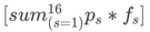
That gives an accuracy of about 58.08% - a little less than the neural network’s mean accuracy, but not enough to confidently say one is better than the other.
However: in this case, categorical accuracy is a misleading metric to use. We’re not refWe don’texpect the 16 previous states to uniquely identify each and every next state, and so we don’t expect very high accuracy.
The issue is that categorical accuracy makes the assumption that all ways of being wrong are equal.5This has nothing to do with our actual goal. So, we have to use a metric that introduces “relative wrongness”.
Imagine you’re trying to predict the rain. If you say you’re 100% sure it’s going to rain tomorrow, and it doesn’t, you’re very clearly wrong. If you say you’re 80% sure it’s going to rain tomorrow, and it doesn’t, you’re still wrong; but you’re less wrong than you would be if you said it with 100% certainty, since at least you allowed for the fact that you might be wrong. In a sense, you’re only 80% wrong.
More technically: consider a single test sample. Let (pi) be our predicted probability that state (i) will be next. Let (yi = 1)
if state (i) is indeed next, and (yi = 0)
otherwise. You can view these as 16 separate predictions. The error for one prediction will be (∣yi − p i∣), and the total absolute error for this sample is 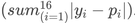
The error for each of the ten neural network variants was computed directly using the test dataset; the results are shown below.
| ID | Mean Absolute Error |
|---|---|
| 31744 | 1.054 |
| 34496 | 1.042 |
| 26420 | 1.055 |
| 90949 | 1.105 |
| 54314 | 1.043 |
| 88775 | 1.033 |
| 83880 | 1.040 |
| 8089 | 1.041 |
| 47680 | 1.048 |
| 89596 | 1.039 |
| Mean | 1.050 |
We calculate this metric for the Markov model using the same framework and assumptions from earlier. If the probability for each next-state (i), given current state (s), is (pis), then the error when that state is chosen when the current state is (s) is clearly (2 ∗ (1 - pis )) . 6If (n is) is the number of times that state (i) follows state (s), then the total error for all current and next states is clearly:
And, for our data, this equals 1.126. In other words, on average, the Markov model is more wrong by about 7.6 percentage points across all categories.
This doesn’t seem like a whole lot, but it’s still an improvement. It validates our intuition - that the larger history that the DNN model uses allows it to be less wrong, on average, even though it’s not able to see every single possible variation.
Since both the categorical accuracy and mean absolute error are superior in the DNN model, we can safely say that it is a superior model.
Finally, we discuss future research that are possible with the same dataset, in the context of continuing to improve the Autoblow AI and sex toys in general.
First: we believe that the procedural generation can be improved. Alternatives to our simple DNN architecture include recurrent neural networks, convolutional neural networks, and generative adversarial networks. We intend to investigate more complex techniques to improve the realism of sequences. However, these need to be balanced against the limitations of physical hardware.
Second: we believe that similar analysis could be applied to other acts and actions depicted in pornography. We focus on blowjobs in order to improve the Autoblow AI, but the fundamental techniques could be used to improve other sex toys.
Third: we would like to extend our investigation to image recognition and video classification. We have already developed a prototype that identifies when a blowjob is present in a still frame, and are in the process of investigating more complex video analysis problems. Particularly, we would like to investigate whether or not it is possible to synchronize a sex toy to unseen pornography.
We look forward to continuing to explore this uncharted space.
To the more technical readers: this is a very simplified version of the actual argument for starting with K–Means. For a longer argument:
It's true that K–Means can be a good starting point, and an easy freebie if your data happens to partition nicely into a set of Voronoi partitions. Our true motivation for using K–Means, though, is quantization (Lloyd's original purpose for the algorithm). In order to build the basic blocks for the Autoblow AI, and to perform the sequencing analysis later, we wanted to reduce the dataset tospecifically sixteen unique points. Therefore, it was appropriate to apply a quantization algorithm. ↩
It's always fun to give context to numbers,so let's do some quick calculations.
Let‘s pretend we’ve got exactly 1 terabyte of main memory to work with (i.e. about the size of an affordable consumer SSD in 2018). We‘ll also assume we’re using a 64–bit computer, and we're therefore using 64–bit floating–point numbers; meaning each next–state probability takes 8 bytes.
So we can store (frac10128=1.25∗1011), or 125 billion, next–states. Using the formula , this corresponds to a maximum current–state length of . In other words, 1 TB of memory lets us handle at most a length–8 current state; for each extra state you multiply that by 16.
At the extreme end,an estimated upper bound for the number of atoms in the universeis KaTeX can only parse string typed expression…which, if you could use each one to store a byte, would let you have a length–67 current–state, which, at 1 second per state, corresponds to just over a minute of porn. ↩
Yes, the usual way of doing text generation is with a recurrent or convolutional neural network. However, a text generator will have to handle possibly millions of possible words, all of which have complex contextual relationships. We only have sixteen “words” in our vocabulary, expressing variations on “go down, then up, or maybe the other way around”. Therefore, it's reasonable to expect good results from a simple model. ↩
This means that, numerically, State 16 is no “farther” from State 1 than it is from 15, which is important. ↩
“If you think that thinking the earth is spherical is just as wrong as thinking the earth is flat, then your view is wronger than both of them put together.” ↩
Or, if it‘s not so clear: because all of the probabilities (pis) for a given current–state (s) must add up to 1, and our truth vector is one–hot encoded, then whatever’s missing from (1−pis) must be in the other categories, and will be counted as error. ↩